
NumPy is primarily used to store and process multi-dimensional array. NumPy is preferred instead of Python List because its performance is better while working on large arrays. NumPy uses fixed (data) types and hence there is no type checking when iterating through objects. NumPy also uses less memory bytes to represent the array in memory and utilizes a contiguous memory, which makes it more efficient to access and process large arrays. NumPy allows insertion, deletion, appending and concatenation, similar to the Python List, but also provides a lot more additional functionality. For an example, NumPy allows to multiple each element of two arrays using a*b were a, b are arrays. NumPy array allows SIMD Vector Processing and Effective Cache Utilization. NumPy is used as a replacement for MatLab, plotting with Matplotlib, images storage and machine learning. NumPy also forms the backend core component for Pandas library.
NumPy is installed using "pip install numpy" command.
NumPy Data Types
NumPy has additional data types compared to the regular Python data types, i.e. strings, integer, float, boolean, complex. The data types is referred using one character, like i for integers, u for unsigned integers etc. Below is a list of all data types in NumPy and the characters used to represent them.
- i - integer
- b - boolean
- u - unsigned integer
- f - float
- c - complex float
- m - timedelta
- M - datetime
- O - object
- S - string
- U - unicode string
- V - fixed chunk of memory for other type ( void )
Arrays
NumPy allows to represent multi-dimensional arrays compared to the built in array module of python which only supports single dimensional arrays. A NumPy array is a grid of values, all of the same type, and is indexed by a tuple of nonnegative integers. The array object in NumPy is called ndarray, it provides a lot of supporting functions that make working with ndarray very easy. Array can be created by passing a list, tuple or any array-like object into the array() method. Methods of creating arrays are array(), linspace(), logspace(), arange(), zeros(), ones(). Arrays can be initialized using nested python lists, and elements can be accessed using square brackets.
Once the array is created, it has many attributes which describe the NumPy array. The shape of an array is the number of elements in each dimension. Shape attribute is represented by the a tuple with each index having the number of corresponding elements, or the size of the array along each dimension. The ndim attribute provides the number of dimensions i.e. the rank of the array.
Once the array is created, it has many attributes which describe the NumPy array. The shape of an array is the number of elements in each dimension. Shape attribute is represented by the a tuple with each index having the number of corresponding elements, or the size of the array along each dimension. The ndim attribute provides the number of dimensions i.e. the rank of the array.
from numpy import *

# Create a rank 1 array i.e. single dimensional array
arr1 = array{[1, 2, 4, 5, 6]}

# Passing a type while creating an array
arr2 = array{[6, 8, 9, 4, 4], int}

arr3 = array([[9.0,8.0,7.0],[6.0,5.0,4.0]])

print(arr1.shape)            # Prints "(5)", means array has 1 dimension which has 5 elements.
print(arr3.shape)            # Prints "(2,3)", means array has 2 dimensions, and each dimension has 3 elements.

print(type(arr1))            # Prints ">class 'numpy.ndarray'<"

print(arr1.ndim)             # Prints number of dimensions in the array

arr1[0] = 5                  # Change an element of the array
Functions to Create Arrays
Numpy also provides many functions to create arrays such as zeros(), ones(), full(), random() which initialize the new array with zeros, ones, other numbers, random values respectively.
# Create an array/matrix of all zeros
np.zeros((2,3))             # 2-Dimensional matrix with all zeros
np.zeros((2,3,3))           # 3-Dimensional matrix with all zeros
np.zeros((2,3,3,2))         # 4-Dimensional matrix with all zeros

# Create an array/matrix of all ones
np.ones((4,2,2))
np.ones((4,2,2), dtype='int32')

# Create an array/matrix with any other constant value
np.full((2,2), 99)          # 2-Dimensional matrix with all 99 number
np.full((2,2), 99, dtype='float32')   # float numbers

# Any other number matrix with full-like shape method
d = np.array([[1,2,3,4,5,6,7],[8,9,10,11,12,13,14]])

np.full_like(d, 4)      # returns array([[4,4,4,4,4,4,4],[4,4,4,4,4,4,4]]) were all values are 4

# alternatively we can use
np.full(a.shape, 4)

# Initialize a matrix of random decimal numbers
np.random.rand(4,2,3)

np.random.rand_sample(d.shape)

# Initialize a matrix of random integer numbers, with range 0 to 7
np.random.randint(7, size=(3,3))

# Initialize random integer numbers, with range -4 to 8
np.random.randint(-4,8, size=(3,3))

# Identity matrix
np.identity(3)                                         # returns array([[1, 0, 0],
                                                       #                [0, 1, 0],
                                                       #                [0, 0, 1]])

arr1 = np.array([1,2,3])

# repeat the array
r1 = np.repeat(arr1, 3, axis=0)                        # returns [1 1 1 2 2 2 3 3 3]

arr2 = np.array([[1,2,3]])
r2 = np.repeat(arr, 3, axis=0)                         # returns [[1 2 3]
                                                       #          [1 2 3]
                                                       #          [1 2 3]]
The arange() method allows to create an array based on numerical ranges. It creates an instance of ndarray with evenly spaced values and returns the reference to it. It takes the start number which defines the first value of the array, and the stop value which defines the end of the array and which isn't included in the array. arrange() method also takes the step argument which defines spacing between two consecutive values, and the dtype which is the type of elements of the output array.
import numpy as np

arr = np.arange(start=1, stop=10, step=3)
print(arr)                           # array([1, 4, 7])

arr = np.arange(start=1, stop=10)
print(arr)                           # array([1, 2, 3, 4, 5, 6, 7, 8, 9])

# starts array from zero and increment each step by one
array = np.arange(5)
print(arr)                           # array([0, 1, 2, 3, 4])

arr = np.arange(5, 1, -1)            # counting backwards
print(arr)                           # array([5, 4, 3, 2])
Datatypes
Every numpy array is a grid of elements of the same type. Numpy provides a large set of numeric datatypes as discussed above that can be used to construct arrays. Numpy tries to guess a datatype when we create an array. The array() function also provides an optional argument 'dtype' to explicitly specify the datatype of the elements. The NumPy array object has a property called dtype that returns the data type of the array.
import numpy as np

a = np.array([1,2,3])

print(a.dtype)            # Prints "int64" i.e. datatype of the array

c = np.array([1,2,3], dtype='S')        # Create array with elements as string data type
c = np.array([1,2,3], dtype='i4')       # Create array with elements as integer with 4 bytes
c = np.array([1,2,3], dtype='int16')    # Create array with elements as integer with 2 bytes

# Get Size
print(a.itemsize)   # prints 4 for int32 element size
print(c.itemsize)   # prints 2 for int16 element size

# Get total size
a.size * a.itemsize   # 1st method
a.nbytes              # 2nd method
Iterating Arrays
Arrays are iterated using regular for loops regardless of their dimensions. NumPy also provides a special nditer() function which helps from very basic to very advanced iterations. It enables to change the datatype of elements while iterating using op_dtypes argument and pass it the expected datatype. An additional argument flags=['buffered'] is passed to provide extra buffer space as data-type change does not occur in place. nditer() also supports filtering and changing the step size. To enumerate the sequence numbers of the elements of the array while iteration, a special ndenumerate() method can be used.
import numpy as np

arr = np.array([[[1, 2], [3, 4]], [[5, 6], [7, 8]]])

for x in arr:
  for y in x:
    for z in y:
      print(z)


# iterating using nditer() function
for x in np.nditer(arr):
  print(x)


for idx, x in np.ndenumerate(arr):
  print(idx, x)
Array Math
Basic mathematical functions operate elementwise on arrays, and are available both as operator overloads and as functions in the numpy module. NumPy allows arithmetic operations on each element of the array.
arr1 = array{[1, 2, 4, 5, 6]}
arr2 = array{[6, 8, 9, 4, 4]}

arr1 = arr1 + 5              # Add 5 to all elements of an array
arr1 += 2                    # Add 2 to all elements of an array
arr1 ** 2                    # Multiply 2 to all elements of an array

# Add elements of two arrays in order. Also called as Vector Operations
arr3 = arr1 + arr2           # returns array { 7, 10, 13, 9, 10 }

print(sqrt(arr1))           # Find square root of each element of the array
print(sin(arr1))            # Find sin value of each element of the array

# Find sum of the array
print(sum(arr1))
print(sort(arr1))
Copy / Clone Array
NumPy allows to copy/clone arrays using the view() function for shallow copy, and the copy() function for deep copy of the array. The copy() function creates a new array while the view() function creates just a view of the original array. The copy owns the data and any changes made to the copy will not affect original array, and any changes made to the original array will not affect the copy. The view does not own the data and any changes made to the view will affect the original array, and any changes made to the original array will affect the view.
a = np.array([1,2,3,4])
# Copy an array arr1 to arr2. The address of both the arrays is same, as both arr1 and arr2 are pointing to same array.
arr2 = arr1

# Clone the array into another array. But its a shallow copy, were elements are still having same address
arr2 = arr1.view()

# Clone the array into another array using deep copy
arr2 = arr1.copy()

# since array arr2 is copy of array arr1, changing arr2 will not change any elements in arr1
arr2[0] = 100
The data type of the existing array can be changed only by making a copy of the array using the astype() method. The astype() function creates a copy of the array, and allows to specify the data type using a string like 'f' for float, 'i' for integer etc as a parameter.
import numpy as np

arr = np.array([1.1, 2.1, 3.1])

newarr1 = arr.astype('i')
newarr2 = arr.astype('int32')
Reorganizing Arrays
The shape of an array is the number of elements in each dimension. NumPy allows to reshape an existing array by allowing to add or remove dimensions or change number of elements in each dimension. NumPy allows to flatten the array i.e. convert a multidimensional array into a 1D array using flatten() function. Alternatively reshape(-1) can also be used to flatten the array. Further Numpy's vstack() function is used to stack the sequence of input arrays vertically to make a single array.
from numpy import *

arr1 = array({
              [1,2,3],
              [4,5,6]
            })

arr1 = array([1, 2, 3, 4, 5, 6, 7, 8, 9, 10, 11, 12])

arr1 = arr1.flatten()            # flatten from multi dimensional to single dimensional array
print(arr1)                      # array([1,2,3,4,5,6])

# reshape single dimensional array to multi dimensional array
newarr = arr.reshape(2, 3, 2)    # The outermost dimension has 2 arrays which contains 3 arrays, each with 2 elements
print(newarr)                    # array([[[ 1  2], [ 3  4], [ 5  6]],  [[ 7  8], [ 9 10], [11 12]]])

before = np.array([[1,2,3,4], [5,6,7,8]])

after = before.reshape((4, 2))                                    # returns [[1 2]
                                                                  #          [3 4]
                                                                  #          [5 6]
                                                                  #          [7 8]]

# Vertically stacking vectors

v1 = np.array([1,2,3,4])
v2 = np.array([5,6,7,8])

np.vstack([v1,v2,v1,v2])                                    # returns array([[1,2,3,4]
                                                            #                [5,6,7,8]
                                                            #                [1,2,3,4]
                                                            #                [5,6,7,8]])

# Horizonral stacking vectors

h1 = np.ones((2,4))
h2 = np.zeros((2,2))

np.vstack([h1,h2])                                    # returns array([[1, 1, 1, 1, 0, 0],
                                                      #                [1, 1, 1, 1, 0, 0]])
Concatenate Arrays
The concatenate() function is used to join the arrays which are joined based on the axis to concatenate along. The arrays are passed to the concatenate() function are as a tuple, which can alternatively be also passed as a Python List. The arrays passed to concatenate() function requires to be of the same data type. Arrays in NumPy have axes which are directions, e.g. axis 0 is the direction running vertically down the rows and axis 1 is the direction running horizontally across the columns. The concatenate() function can operate both vertically and horizontally based on the axis argument specified. If we set axis = 0, the concatenate function will concatenate the NumPy arrays vertically which is also the default behavior if no axis is specified. On the other hand, if we manually set axis = 1, the concatenate function will concatenate the NumPy arrays horizontally.
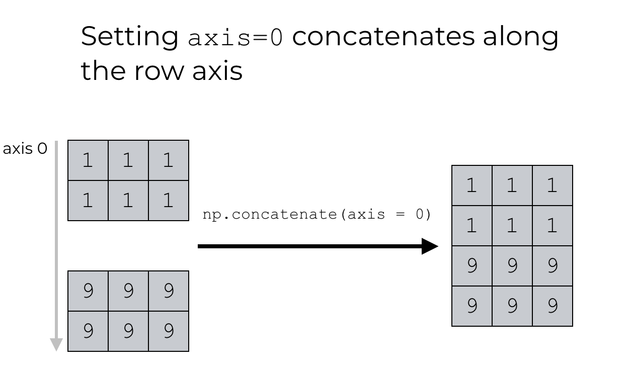

import numpy as np

arr1 = np.array([[1, 2], [3, 4]])
arr2 = np.array([[5, 6], [7, 8]])

arr = np.concatenate((arr1, arr2), axis=0)
print(arr)                                              # array([[1,2], [3,4], [5,6], [7,8]])

arr = np.concatenate((arr1, arr2), axis=1)
print(arr)                                              # array([[1,2,5,6], [3,4,7,8]])
Stacking
Stacking is similar as concatenation, the only difference is that stacking is done along a new axis. A sequence of arrays to be joined are passed to the stack() method along with the axis. If axis is not explicitly passed it is taken as 0. NumPy provides helper functions such as hstack() to stack along rows, vstack() to stack along columns and dstack() to stack along height i.e. depth.
import numpy as np

arr1 = np.array([1, 2, 3])
arr2 = np.array([4, 5, 6])

arr = np.stack((arr1, arr2), axis=1)
print(arr)

arr = np.hstack((arr1, arr2))
print(arr)

arr = np.vstack((arr1, arr2))
print(arr)

arr = np.dstack((arr1, arr2))
print(arr)
Splitting Array
The array_split() function takes an array and number of split as arguments to break the array into multiple parts.
import numpy as np

arr = np.array([1, 2, 3, 4, 5, 6])

newarr = np.array_split(arr, 4)
print(newarr)

arr = np.array([[1, 2, 3], [4, 5, 6], [7, 8, 9], [10, 11, 12], [13, 14, 15], [16, 17, 18]])

newarr = np.array_split(arr, 3)
print(newarr)

newarr = np.array_split(arr, 3, axis=1)
print(newarr)
Searching Arrays
The where() method allows to search an array for a certain value, and return the indexes for the matched elements. Another method called searchsorted() performs a binary search in the array, and returns the index where the specified value would be inserted to maintain the search order. The searchsorted() method starts the search from the left by default and returns the first index where the argument number is no longer larger than the next value. By specifying the argument side='right' it allows to return the right most index instead.
import numpy as np

arr = np.array([1, 2, 3, 4, 5, 4, 4])

x = np.where(arr == 4)
print(x)

x = np.where(arr%2 == 0)
print(x)

arr = np.array([1, 3, 5, 7])

x = np.searchsorted(arr, 3)
print(x)

x = np.searchsorted(arr, [2, 4, 6])
print(x)
NumPy's all() method tests all the array elements along a given axis if it evaluates to True. The any() method tests any array element along a given axis if it evaluates to True. In other words, numpy.any() method returns True if at least one element in an array evaluates to True while numpy.all() method returns True only if all elements in a NumPy array evaluate to True. NumPy also allows conditional operators to check the condition on each element of the array, and allows to 'and'/'or' the boolean arrays to get a cumulative result.
import numpy as np

arry = np.array([1, 2, 73, 4, 5, 89, 54, 34, 102])

# Find any value in the column has a value which is greater than 50
x = np.any(arry > 50, axis=0)
print(x)                                     # True

#Find the columns which has all the values that are grater than 50
x = np.all(arry > 50, axis=0)
print(x)                                     # False

#Find the rows which has all the values that are grater than 50
x = np.all(arry > 50, axis=1)
print(x)                                     # True

# Find values in array greater than 50 and less than 100
x = ((arry > 50) & (arry < 100))
print(x)                                     # [False, False, True, False, False, True, True, False, False]

# negation of above condition
x = (~((arry > 50) & (arry < 100)))
print(x)                                     # [True, True, False, True, True, False, False, True, True]
Sorting Arrays
Arrays can be sorted in numeric or alphabetical order with ascending or descending order.
import numpy as np

arr = np.array([[3, 2, 4], [5, 0, 1]])

print(np.sort(arr))

arr = np.array(['banana', 'cherry', 'apple'])

print(np.sort(arr))
Filtering Arrays
NumPy allows to filter an array using a list of booleans corresponding to indexes in the array. If the value at an index is True that element is contained in the filtered array, otherwise when False it is excluded from the filtered array. The filtered array can be created by hardcoding True/False values, or using a filter variable as a substitute for the filter array.
import numpy as np

arr = np.array([41, 42, 43, 44])

x = [True, False, True, False]

newarr = arr[x]
print(newarr)

filter_arr = arr > 42

newarr = arr[filter_arr]
print(newarr)
NumPy ufuncs
Computation of NumPy arrays is enhanced when used the vectorized operations, generally implemented through NumPy's universal functions (ufuncs). Vectorized operation simply performs an operation on the array, which will then be applied to each element. Such vectorized approach is designed to push the loop of processing each array element into compiled layer of NumPy, which leads to much faster execution. Vectorized operations in NumPy are implemented via ufuncs, whose main purpose is to quickly execute repeated operations on values in NumPy arrays. Computations using vectorization through ufuncs are nearly always more efficient than their counterpart implemented using Python loops, especially as the arrays grow in size.
Ufuncs exist in two flavors, unary ufuncs which operate on a single input, and binary ufuncs which operate on two inputs. ufuncs usually take array under operation along with additional arguments such as 'where' which is a boolean array or condition, 'dtype' which defines the return type of elements and 'out' which is the output array where the return value could be copied. Below are wide range of examples of ufuncs.
Ufuncs exist in two flavors, unary ufuncs which operate on a single input, and binary ufuncs which operate on two inputs. ufuncs usually take array under operation along with additional arguments such as 'where' which is a boolean array or condition, 'dtype' which defines the return type of elements and 'out' which is the output array where the return value could be copied. Below are wide range of examples of ufuncs.
# Array Arithmetic Operations

x = np.arange(4)
print("x     =", x)
print("x + 5 =", x + 5)
print("x - 5 =", x - 5)
print("x * 2 =", x * 2)
print("x / 2 =", x / 2)
print("x // 2 =", x // 2)  # floor division
print("-x     = ", -x)
print("x ** 2 = ", x ** 2)
print("x % 2  = ", x % 2)

# Absolute Value

x = np.array([-2, -1, 0, 1, 2])
abs(x)

# Trigonometric functions

theta = np.linspace(0, np.pi, 3)
print("theta      = ", theta)
print("sin(theta) = ", np.sin(theta))
print("cos(theta) = ", np.cos(theta))
print("tan(theta) = ", np.tan(theta))

# Exponents and Logarithms

x = [1, 2, 3]
print("x     =", x)
print("e^x   =", np.exp(x))
print("2^x   =", np.exp2(x))
print("3^x   =", np.power(3, x))
print("ln(x)    =", np.log(x))
print("log2(x)  =", np.log2(x))
print("log10(x) =", np.log10(x))

# Aggregates

x = np.arange(1, 6)
np.add.reduce(x)         # reduce repeatedly applies a given operation to the elements of an array until only a single result remains.
np.multiply.reduce(x)

np.add.accumulate(x)     # stores all the intermediate results of the computation
Boolean Masking and Advance Indexing
Masking in python and data science is when you want manipulated data in a collection based on some criteria. Masking allows to extract, modify, count, or otherwise manipulate values in an array based on some criterion. NumPy enables boolean masking to create a special type of array called Masked Array. A masked array is created by applying scalar (conditional operator) to NumPy array.
# Load Data from File containing (1,2,73,4,5,89...)
filedata = np.genfromtext('data.txt', delimiter=',')

filedata > 50
# returns array([[False, False, True, False, False, True]])

# Index using the condition, i.e. grab the value if its greater than 50
filedata[filedata > 50]
# returns array([73, 89])

# We can pass index as a list to fetch values in NumPy
g = np.array([1,2,3,4,5,6,7,8,9])
g[[1,2,8]]  # returns array([2, 3, 9])

# Pass multiple array index for each dimension
k = np.array([[1,2,3], [4,5,6], [7,8,9]])
k[[1,2],[2,2]]
# returns array([6, 9])

# another example with slicing
k[[1,2], 3:]
Matrix
Matrix module contains the functions which return matrices instead of arrays. It contains functions which represent arrays in matrix format. A matrix is a specialized 2-D array in NumPy that retains its 2-D nature through operations. It has certain special operators, such as * (matrix multiplication) and ** (matrix power). The matrix() function returns a matrix from an array of objects or from the string of data. The asmatrix function interprets the input as matrix. The methods zeros(), ones(), rand(), identity() and eye() returns matrix with zeros, ones, random values, square identity matrix and matrix with ones on diagonal respectively.
arr1 = array({ [1,2,3], [4,5,6] })
m1 = matrix(arr1)                # convert 2D array to a matrix
m2 = matrix('1 3 6 : 4 6 7')     # create matrix
m2.diagonal()                    # returns diagonal elements in the matrix
m3  = m1 * m2                    # multiply matrices
Slicing
Slicing in python means taking elements from one given index to another given index. Similar to Python lists, numpy arrays can be sliced. Since arrays may be multidimensional, you must specify a slice for each dimension of the array. Slice is represented instead of index like [start:end:step]. The default values for start is 0, end is the length of the array in that dimension and step is 1. Negative slicing is achieved by using the minus operator to refer to an index from the end.
d = np.arrary([[1,2,3,4,5,6,7],[8,9,10,11,12,13,14]])

# Get a specific element [r, c]
d[1, 5]  # returns 13
d[1, -2] # returns 13

# Get a specific row
d[0, :]

# Get a specific column
d[:, 2]

# Getting [startindex:endindex:stepsize]
d[0, 1:6:2]     # get elements between 2nd and 7th with alternate numbers
d[0, 1:-1:2]

# Change value of the element
a[1,5] = 20

# Set value of 3rd column to 5
a[:,2] = 5

a[:,2] = [1,2]

e = np.array([[[1,2],[3,4]],[[5,6],[7,8]]])

# Get specific element (work outside in)
b[0,1,1] = 4

b[:,1,:]    # returns array([[3,4], [7,8]])

# Replace values in 3-dimensional array
b[:,1,:] = [[9,9],[8,8]]

# Returns array([[[1,2],[9,9]],[[5,6],[8,8]]])
Generate Random Number
NumPy offers the random module to work with random numbers. The randint() function when passed the integer will generate a random number from 0 until the integer argument. It also takes a size parameter which specifies the shape of an array, in order for randint() to return a multi-dimensional array of random integers. NumPy also has the choice() method which allows to generate a random value based on an array of values.
from numpy import random

print(random.randint(100))     # random integer between 0 to 100

print(random.rand())     # random float between 0 and 1

x=random.randint(100, size=(5))
print(x)                # prints an array containing 5 random integers from 0 to 100

x = random.randint(100, size=(3, 5))
print(x)                 # prints 2-D array with 3 rows, each row containing 5 random integers from 0 to 100

x = random.choice([3, 5, 7, 9])
print(x)                 # prints one of the values randomly from the passed array

x = random.choice([3, 5, 7, 9], size=(3, 5))
print(x)                 # prints 2-D array with 3 rows, each row containing 5 values from passed array
Linear Algebra
NumPy package contains numpy.linalg module that provides all the functionality required for linear algebra. Below are some of the important functions in this module.
dot: It returns the dot product of two arrays. For 2-D vectors, it is the equivalent to matrix multiplication. For 1-D arrays, it is the inner product of the vectors. For N-dimensional arrays, it is a sum product over the last axis of a and the second-last axis of b.
vdot: It returns the dot product of the two vectors. If the first argument is complex, then its conjugate is used for calculation. If the argument id is multi-dimensional array, it is flattened.
inner: It returns the inner product of vectors for 1-D arrays. For higher dimensions, it returns the sum product over the last axes.
outer: Returns the outer product of two vectors.
matmul: It returns the matrix product of two 2-D arrays. For arrays with dimensions above 2-D, it is treated as a stack of matrices residing in the last two indexes and is broadcast accordingly.
determinant: It calculates the determinant from the diagonal elements of a square matrix. For a 2x2 matrix [[a,b], [c,d]], the determinant is computed as ‘ad-bc’. The larger square matrices are considered to be a combination of 2x2 matrices.
solve: It gives the solution of linear equations in the matrix form.
inv: It calculates the inverse of a matrix. The inverse of a matrix is such that if it is multiplied by the original matrix, it results in identity matrix.
dot: It returns the dot product of two arrays. For 2-D vectors, it is the equivalent to matrix multiplication. For 1-D arrays, it is the inner product of the vectors. For N-dimensional arrays, it is a sum product over the last axis of a and the second-last axis of b.
import numpy.matlib
import numpy as np

a = np.array([[1,2],[3,4]])
b = np.array([[11,12],[13,14]])
np.dot(a,b)                        # returns [[37,40], [85,92]]
vdot: It returns the dot product of the two vectors. If the first argument is complex, then its conjugate is used for calculation. If the argument id is multi-dimensional array, it is flattened.
import numpy as np
a = np.array([[1,2],[3,4]])
b = np.array([[11,12],[13,14]])
print np.vdot(a,b)                  # prints 130
inner: It returns the inner product of vectors for 1-D arrays. For higher dimensions, it returns the sum product over the last axes.
import numpy as np
a = np.array([[1,2], [3,4]])
b = np.array([[11, 12], [13, 14]])

print np.inner(a,b)        # returns   [[35 41]
                           #            [81 95]]
outer: Returns the outer product of two vectors.
matmul: It returns the matrix product of two 2-D arrays. For arrays with dimensions above 2-D, it is treated as a stack of matrices residing in the last two indexes and is broadcast accordingly.
import numpy.matlib
import numpy as np

a = [[1,0],[0,1]]
b = [[4,1],[2,2]]
print np.matmul(a,b)        # returns   [[4  1]
                            #            [2  2]]
determinant: It calculates the determinant from the diagonal elements of a square matrix. For a 2x2 matrix [[a,b], [c,d]], the determinant is computed as ‘ad-bc’. The larger square matrices are considered to be a combination of 2x2 matrices.
import numpy as np

a = np.array([[1,2], [3,4]])
print np.linalg.det(a)               # returns -2.0
solve: It gives the solution of linear equations in the matrix form.
inv: It calculates the inverse of a matrix. The inverse of a matrix is such that if it is multiplied by the original matrix, it results in identity matrix.
import numpy as np
a = np.array([[1,1,1],[0,2,5],[2,5,-1]])

ainv = np.linalg.inv(a)
print(ainv)
Statistics
Numpy supports various statistical calculations using the various functions that are provided in the library like Order statistics, Averages and variances, correlating, Histograms. NumPy has a lot in-built statistical functions such as Mean, Median, Standard Deviation and Variance.
x = [32.32, 56.98, 21.52, 44.32, 55.63, 13.75, 43.47, 43.34]

# Functions to Find Mean, Median, SD and Variance

mean = np.mean(X)
print("Mean", mean)                  # 38.91625

median = np.median(X)
print("Median", median)              # 43.405

sd = np.std(X)
print("Standard Deviation", sd)      # 14.3815654029

variance = np.var(X)
print("Variance", variance)          # 206.829423437

# Functions to Find Min, Max and Sum

stats = np.array([[1,2,3], [4,5,6]])

np.min(stats)                        # returns 1
np.min(stats, axis=0)                # returns [1, 2, 3]  as all the minimum values in top row

np.max(stats, axis=1)                # returns [3, 6]

np.sum(stats)                        # adds all elements and returns 21
np.sum(stats, axis=0)                # adds columns and returns array([5, 7, 9])
Histograms
NumPy has a numpy.histogram() function that is a graphical representation of the frequency distribution of data. The histogram() function mainly works with bins i.e. class intervals and set of data given as input. The numpy.histogram() function takes the input array and bins as two parameters. The successive elements in bin array act as the boundary of each bin. Numpy histogram function will give the computed result as the occurrances of input data which fall in each of the particular range of bins. That determines the range of area of each bar when plotted using matplotlib. Matplotlib enables to convert the numeric representation of histogram into a graph. The plt() function of pyplot submodule takes the array containing the data and bin array as parameters and converts into a histogram.
import numpy as np
from matplotlib import pyplot as plt

arr = np.array([22,87,5,43,56,73,55,54,11,20,51,5,79,31,27])
# returns (array([3, 4, 5, 2, 1]), array([  0,  20,  40,  60,  80, 100]))

hist = np.histogram(arr, bins=[0,20,40,60,80,100])

plt.hist(arr, bins=[0,20,40,60,80,100])
plt.title("histogram")
plt.show()
No comments:
Post a Comment